Analyzing Real-Time Systems
In a previous post (here) we discussed what are and the types of real-time systems. We also gave some examples to highlight their importance and clarify some of the confusion regarding the real-time and run-time performance tradeoff. In this post, we will focus exclusively on “hard” real-time systems and how they are statically analyzed (i.e. before the program is run) to guarantee that deadlines are never missed.
NOTE: You can find a great survey of hard real-time analysis methods and tools (both commercial and open-source) here. I will only discuss one method in this post, but there are alternatives.
Overview
Our goal is to ensure that the hard real-time system never misses a deadline. To achieve that, we are going to count how many clock cycles the processor will take to run our given hard real-time program through any possible execution path. Then we will select the code path that takes the longest to run and declare that our Worst-Case Execution Time (WCET). The hard real-time system will meet all its deadlines if the WCET is smaller than the deadline, otherwise the system needs to be re-designed so that it does meet its deadlines. For example, the WCET to draw a frame must be less than 16 ms if we would like the Chrome browser to operate at 60 fps although that is not a hard real-time application!
NOTE: I do mean counting how many clock cycles it takes to execute each add, sub, ld, st, etc instruction. For this reason, I have sometimes heard people call this method cycle-counting analysis.
The worst-case idea is actually very important and perhaps the most troublesome in this analysis. For example, the WCET of an if-statement is given by the branch with the longest run-time. And this is regardless of how often that particularly long-running branch of the if-statement is executed because in practice it is hard to know how many times this branch is run. So our estimated program run-time can add up in unrealistic ways when the code has widely different best-case and worst-case execution times!
Lets consider the simple pseudo-code example below to nail down this idea. The
for-loop executes the if-statement N times and the run-times of statements
A and B are 2 ms and 10 ms respectively. So the WCET for this code is 10 * 10
ms = 100 ms because we assume that the program is invariably going to execute
the worst-case branch B from the if-statement. However, it might be the case
that B is only executed 50% of the time on average, so a more realistic
run-time for this code would be 5 * 2 ms + 5 * 10 ms = 60 ms. Even in this
simple example we are over-estimating the WCET by about 40%! But we cannot
improve our WCET with the information provided because we have no idea how
frequently x(i) evaluates to true or false. If we heavy-handedly assumed that
x(i) is true say 50% of the time, but its actually 60% or 70% in practice, we
are at risk of missing deadlines.
for (i = 0; i < N; ++i)
    if x(i)
        A
    else
        B
It is for these reasons that we can often hear engineers saying that caching and other hardware optimization features are incompatible with hard real-time analysis. The idea of caching is to use smaller and faster memories close to the processor to reduce the time it takes to load or store data. However, caching makes the run-time of load and store instructions difficult to estimate because we cannot tell whether a memory access will result in a cache hit, so it has short run-time, or a miss so we need to check slower memories which takes longer. Therefore, the real-time analysis must often assume that the caches will miss, since this is the worst-case, and the overall WCET estimate will be far detached from the real run-time.
NOTE: As far as I know, hard real-time systems often rely on small processors, like the ARM Cortex-M0, or processors with relatively simple pipelines and caches because these are easier to analyze. For example, you can see this list of targets supported by a commercial real-time analysis tool. There is also extensive research to try to account for more complex processors, but I have not looked much into it.
In summary, we would like to make WCET analysis easier for ourselves to check whether the system will meet its deadlines. We can do so by ensuring that the program’s worst-case and best-case run-times are not outrageously different. We can also use simpler processors that do not have complicated features, like caching, that introduce unpredictability in the run-time of instructions. And without further ado, lets analyze a simple program to see how WCET works. We will perform the analysis in two steps:
- Control Flow Graph (CFG) construction
- Implicit Path Enumeration (IPET)
Control Flow Graph
We will analyze the following C program that implements bubblesort to sort 10 integers. I took this code from the BEEBS benchmarks mostly because it is relatively straight-forward to analyze.
#define FALSE 0
#define TRUE 1
#define NUMELEMS 10

void BubbleSort(int Array[]) {
    int Sorted = FALSE;
    int Temp, Index, i;

    for (i = 0; i < NUMELEMS; i++) {
        Sorted = TRUE;
        for (Index = 0; Index < NUMELEMS; Index++) {
            if (Index >= NUMELEMS - i) {
                break;
            }
            if (Array[Index] > Array[Index + 1]) {
                Temp = Array[Index];
                Array[Index] = Array[Index + 1];
                Array[Index + 1] = Temp;
                Sorted = FALSE;
            }
        }

        if (Sorted) {
            break;
        }
    }
}
The C code above is there mostly for illustration purposes because we are
actually interested in the disassembly of that program’s binary. Analysing the
disassembly, as opposed to the C code, takes into account any optimizations and
transformations introduced by the compiler, so we eliminate potential errors in
our estimation. In this case, it looks like the compiler inlined the
BubbleSort function into another function called benchmark to produce the
code shown below. The program was compiled with LLVM 10 for the ARMv6-M
architecture.
00000074 <benchmark>:
  74:	b5f0      	push	{r4, r5, r6, r7, lr}
  76:	2000      	movs	r0, #0
  78:	2164      	movs	r1, #100	; 0x64
  7a:	4a0d      	ldr	r2, [pc, #52]	; (b0 <benchmark+0x3c>)
  7c:	6813      	ldr	r3, [r2, #0]
  7e:	2601      	movs	r6, #1
  80:	460c      	mov	r4, r1
  82:	4615      	mov	r5, r2
  84:	e006      	b.n	94 <benchmark+0x20>
  86:	602f      	str	r7, [r5, #0]
  88:	606b      	str	r3, [r5, #4]
  8a:	2600      	movs	r6, #0
  8c:	1e64      	subs	r4, r4, #1
  8e:	1d2d      	adds	r5, r5, #4
  90:	2c00      	cmp	r4, #0
  92:	d004      	beq.n	9e <benchmark+0x2a>
  94:	686f      	ldr	r7, [r5, #4]
  96:	42bb      	cmp	r3, r7
  98:	dcf5      	bgt.n	86 <benchmark+0x12>
  9a:	463b      	mov	r3, r7
  9c:	e7f6      	b.n	8c <benchmark+0x18>
  9e:	2e00      	cmp	r6, #0
  a0:	d103      	bne.n	aa <benchmark+0x36>
  a2:	1e49      	subs	r1, r1, #1
  a4:	1c40      	adds	r0, r0, #1
  a6:	2864      	cmp	r0, #100	; 0x64
  a8:	d1e8      	bne.n	7c <benchmark+0x8>
  aa:	2000      	movs	r0, #0
  ac:	bdf0      	pop	{r4, r5, r6, r7, pc}
  ae:	46c0      	nop			; (mov r8, r8)
  b0:	00000164 	.word	0x00000164
The first step in the analysis is to construct a Control Flow Graph (CFG) out of this disassembly. The CFG is a directed graph representation that captures the control-flow information, i.e. branches, conditionals, loops, etc, from the program. The nodes of a CFG represent blocks of code without branches or branch destinations, while the edges are branches as shown in the figure below. Each node and edge is given an identifier (e.g. block0 or b0 for short, e0, b1, etc) for convenience and a cost coefficient.
The cost coefficient represents the worst-case cost, in clock cycles, of executing the sequence of instructions in a node’s block of code. And this is where the choice of processor is very important! A cost model of the chosen processor is used to estimate the time that the microarchitecture takes to execute each instructions. From this, we calculate each node and edge’s cost coefficient. If the processor has unpredictable features like complex caching then its hard to approximate the worst-case run-time of instructions, and as a result, the cost cofficients could be way off-board.
In our case, the cost model is very simple because hard real-time analysis
targets a processor similar to an ARM Cortex-M0 which has a very simple
microarchitecture with the very predictable execution times listed
here.
For example, node b6 has a compare (cmp) instruction followed by a
conditional branch (bne) with 1 and 3 clock cycles of run-time respectively,
so the cost coefficient for b6 is 1 + 3 = 4.
NOTE: I generated this CFG using a tool I jointly developed with a colleague during my PhD. It takes an ARMv6-M program binary as an input along with a configuration file to produce the WCET estimate (among other things like the CFG!). The tool is open-source and is available here.
NOTE: CFG’s are not unique to real-time analysis. They are used in many other applications like compilers.
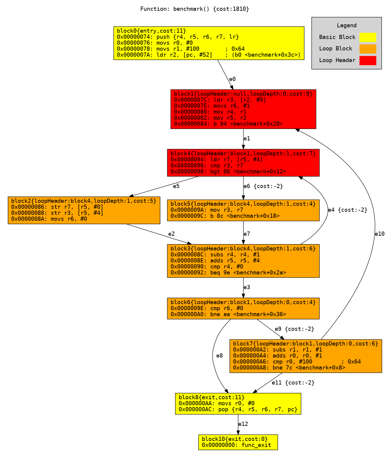
Control Flow Graph for the bubblesort program. block0 is the start of the function. block10 is a placeholder exit node to ensure that the CFG has a single exit point. The exit node has no "cost" because it does not include any real instructions.
Integer Linear Programming
The second part of the analysis uses Implict Path Enumeration (IPET) to calculate the WCET. IPET derives an Integer Linear Programming (ILP) problem by combining the flow information and coefficients encoded in the CFG. It consists of an objective function, that encodes the run-time of the code when solved, and a set of constraints over the variables in that function.
The ILP problem for our bubblesort CFG is shown below. It tells us that the
run-time of the code will be 11 clock cycles (i.e. b0’s cost coefficient)
multiplied by the number of times that node b0 in the CFG is executed plus 9
clock cycles multiplied by the number of times that node b1 is executed and so
on. But the ILP also gives us a few restrictions or contraints when calculating
a solution for the variables b0, b1, e4, e6, etc. For example, there is an
input constraint b0 = 1 meaning that the code at node b0 can only be executed
once on entry to the function which makes sense because that code is not within
a loop. There is also an output constraint b0 = e0 restricting edge e0 to be
“executed” as many times as the code at b0 is executed.
The ILP formulation is constructed from a simple graph traversal of the CFG. Each node and edge has a cost coefficient (or 0) and a unique identifier; the objective function is a summation of these terms. The majority of the constraints relate the number of times that the edges are followed with how often the node is executed. Loop bounds are the only constraints that are difficult to construct as the information is not readily available in the CFG, so these bounds are either input manually or estimated automatically using a tool like SWEET.
/* Objective function */
max: 11 b0 + 9 b1 + 5 b2 + 6 b3 + 7 b4 + 4 b5 + 4 b6 + 6 b7 + 11 b8 + 0 b10
     - 2 e4 - 2 e6 - 2 e9 - 2 e11;

/* Output constraints */
b0 = e0;
b1 = e1;
b2 = e2;
b3 = e3 + e4;
b4 = e5 + e6;
b5 = e7;
b6 = e8 + e9;
b7 = e10 + e11;
b8 = e12;
b10 = 1;

/* Input constraints */
b0 = 1;
b1 = e0 + e10;
b2 = e5;
b3 = e2 + e7;
b4 = e1 + e4;
b5 = e6;
b6 = e3;
b7 = e9;
b8 = e8 + e11;
b10 = e12;

/* Loop constraints */
10 b0 <= b1;
b1 <= 10 b0;
10 b1 <= b4;
b4 <= 10 b1;
Finally, we need to solve the ILP problem by maximizing the objective function as we would like to calculate the worst-case execution time. We can do just that with a nice tool called lp_solve that you probably have installed in your Linux computer without realizing. The lp_solve output for our bubblesort ILP is shown below, so the WCET estimate for this code is 1810 clock cycles!
Value of objective function: 1810.00000000

Actual values of the variables:
b0                              1
b1                             10
b2                            100
b3                            100
b4                            100
b5                              0
b6                             10
b7                             10
b8                              1
b10                             1
e4                             90
e6                              0
e9                             10
e11                             1
e0                              1
e1                             10
e2                            100
e3                             10
e5                            100
e7                              0
e8                              0
e10                             9
e12                             1
Conclusion
And that is it! We statically analyzed a hard real-time implementation of bubblesort and estimated a WCET. It is worth pointing out that this is frustratingly difficult in practice as the complexity of the problem increases very quickly when programs are larger or the processor has more features. Also, there is a lot of manual labour involved in getting the right parameters, like look bounds, and constantly re-designing bits of your system to try to fulfil the real-time constraints. But hopefully this was a helpful introduction to hard real-time systems!